Hazard Assessment

Background filters

New background filters have been added to the Hazard Assessment application. The time of day filter can be used to see the effect of removing events during blasting/shift change on the hazard results. You can either view the results in raw or normalised form. The hazard calculations do normalisation for the event rate calcs anyway, to represent hazard in yearly terms. If your analysis period is six months, the number of events is doubled to represent a year's worth of events. When applying the time-of-day filter though, the actual analysis period is less than six months, because several hours per day have been removed. Without normalisation, the hazard should always drop when applying the time-of-day filter, because you are removing events, and nothing else changes (i.e. still using 6 months). If normalisation is turned on, the time period that has been removed is accounted for in the hazard calculations. The results then represent accurately the state of the hazard during the relevant times of day.

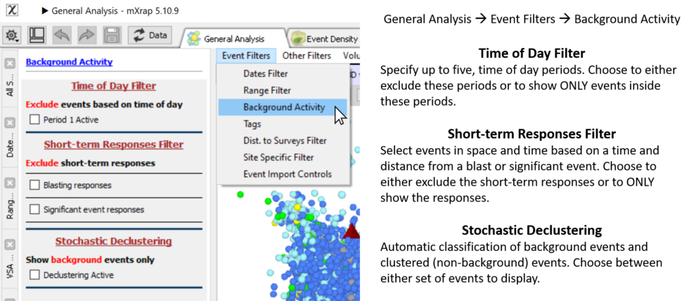
We have added some new event filter options to general analysis related to 'background' activity. 'Background' events are generally defined as having low variability in space and time. The new background filters aim to identify events that are clustered in space and time and the user can either display the 'clustered' or the 'background' component of seismicity.

There are three ways of classifying clustered events; by time-of-day, by proximity to blasts and significant events, and by a stochastic declustering procedure. Stochastic declustering will be explained in a separate blog post.

With the time-of-day filter, you can specify up to five periods of the day, to define increased activity around shift change/blasting times. Times are entered in hours, e.g. 5:30pm = 17.5. Events within these periods will not be shown by default but you can toggle/invert the time-of-day filter to only show events inside the time-of-day periods (and hide events outside).

With the short-term responses filter, you can define a time period and spherical radius around blasts and significant events to filter out events. Use the normal blast filter to control which blasts are considered. Significant events are considered if they are within the current base filter, and above the specified magnitude. Note that the significant event itself is not filtered out (it is treated as a background event, not a clustered event). Just like the time-of-day filter, you can toggle/invert the filter to only show the responses, and hide events outside the response windows.

The last filter option is an automatic classification system for separating background and clustered events. You can toggle between each component of seismicity defined from stochastic declustering. Watch out for the next blog post if you are interested in the details of how this method works.

This is a new addition to the General Analysis application. Find the panel under 'Event Filters / Background Activity'.

Short-term Responses

Normalisation also applies to the short-term responses filter, where events can be removed based on a time and distance from a blast or significant event. In this case the normalisation is a bit more complicated. With the time-of-day filter, the effective analysis period is the same for the whole grid. In this case however, there will be an uneven distribution of space and time removed from the analysis. So, each individual cell has its own effective analysis period, based on how many triggers (and responses) are nearby. The idea is still the same though, without normalisation, the hazard will drop due to the removal of events without adjusting the analysis period. With normalisation turned on, the results will represent the hazard state outside of short-term response regions.

A new chart has been added to the Hazard Assessment app that shows the effect of different short-term response filtering on hazard. The chart works in a similar way as the Track Volumes over Time chart, by computing the hazard over and over again, automatically changing variables with each run. The chart and associated control panel can be found in the Hazard Assessment / Hazard ISO's window, under the Response Analysis menu. To generate the chart, you need to specify a maximum response time, a time delta, and response distances (up to 6). The hazard will be calculated for each response distance and for each response time from zero to the maximum (at delta intervals). The hazard recorded is the probability of exceeding the design magnitude within the chosen grid, which is the value displayed in the footer of the 3D ISO view. It can take some time to calculate, depending on how many iterations you specify. The video below shows the chart being generated for response times up to 72 hours and response distances of 50, 100 and 150 m.

We have added some new features to the Hazard Assessment app to calculate the minode hazard for filter volumes. This works just like the current minode calculations, where you can select minodes and compute the probability, P, of exceeding your design magnitude, within R of any selected minodes. The volume hazard refers to the seismic hazard for minodes within the filter volume. The same backdate, backrange, Mdesign and R parameters apply as the existing tools.

Another tool has been added to track the volume hazard over time. Essentially this repeats the volume hazard calculations, stepping the backdate through time and plotting the hazard per volume. Refer to the 'Track Volume Hazard' training video for a walkthrough of the new tools in the hazard app.

Event Rate

The Hazard Assessment application uses a grid-based approach to describe the seismic hazard throughout your mine. Each grid point essentially represents a seismic source with a specific frequency-magnitude relationship. A frequency-magnitude relationship is defined from the $M_{UL}$, $Mmin$, $b$-value, and event rate. We've previously delved into $M_{UL}$ in this post. We also discussed how $Mmin$ and $b$-value are calculated along with other gridding parameters in this post. The event rate is something we haven't taken a dive into yet, so we'll get into it in this post.

Event rate sounds like a simple calculation but there are quite a few complexities worth explaining here. There are also a couple of controls for event rate hidden away in the Advanced Tools that might be worth investigating at your site. These controls will be explained below too.

The event rate refers to the number of events above a certain reference magnitude, usually $Mmin$. On the frequency-magnitude chart, essentially the $b$-value is the slope and event rate is the intercept. It is related to the a-value of the Gutenberg-Richter distribution. You might also see the event rate referred to as the lambda (λ) value. This comes from the Poisson distribution where λ is the rate parameter.

The event rate parameter refers to a specific time interval and volume. The number of events during the data period is adjusted to refer to one year's worth of activity. For the hazard calculations, the event rate is associated with the number of events within the 3D cubic volume of the grid cell. However, the event rate that is plotted in 3D with isosurfaces is adjusted to refer to the event rate within a 50 m spherical volume. The standard volume adjustment is done so that you can modify the grid spacing and the event rate will remain the same.

Event Splattering

Events within the data period are assigned to the grid with a 'splattering' process. Just like if you throw a ripe tomato, it might splatter onto the wall, events are splattered onto its nearby grid points. The kernel function controls the distribution of an event onto the grid. Grid cells closer to the event have a higher weighting. A cubic kernel function is used to assign a portion of each event to grid points within a maximum radius, Rmax. The total contribution of a single event to the grid is always normalised to be equal to one. This avoids the problem of overcounting or undercounting events and ending up with an inaccurate grid event count. If you have 1,000 events in the data period, you want the total event count of the grid points to also work out to 1,000. When all events have been splattered, each grid point then has the number of events associated with its cubic volume.

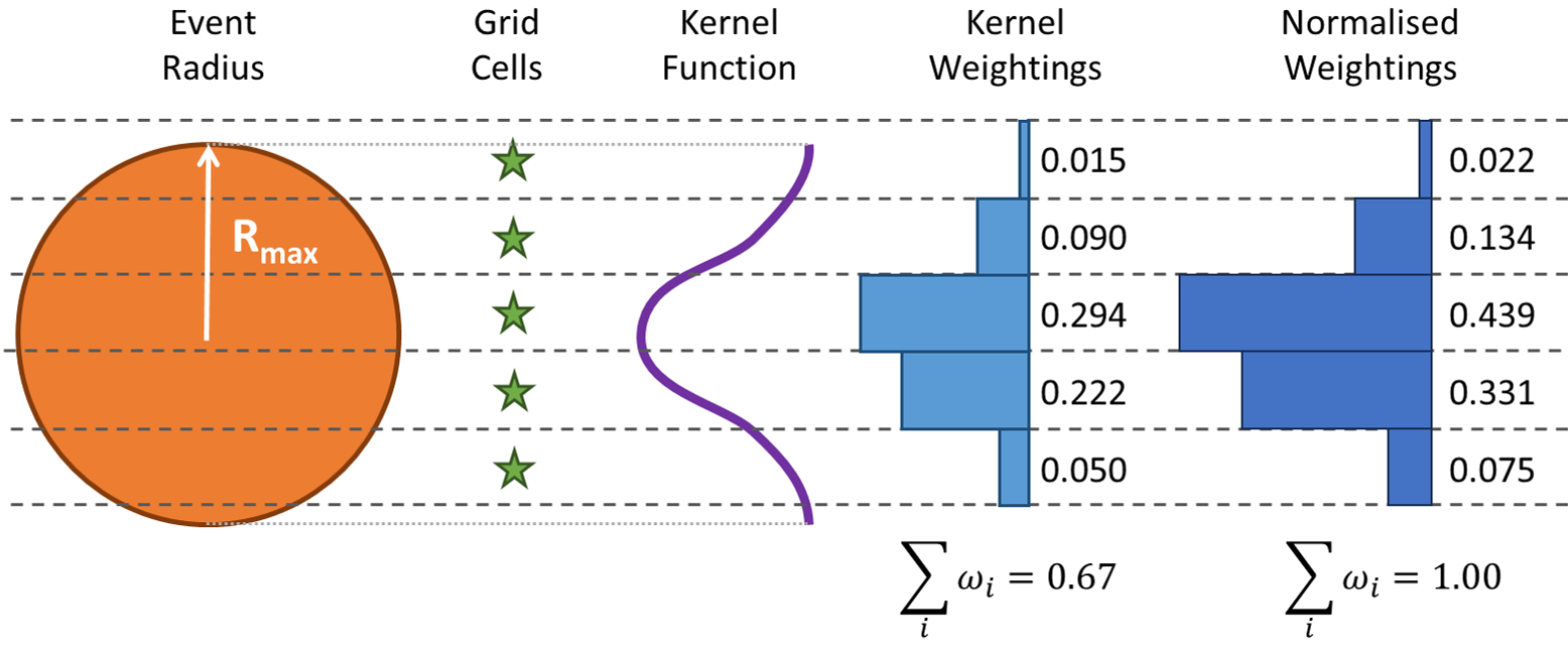
The maximum radius, Rmax, of the kernel function is adjusted for each event. Larger magnitude events have a bigger area of influence. The radius is also expanded in lower density areas to reduce the artifacts around the edges of seismic clusters. The Rmax is generally the maximum of the following parameters:

• 20 m. Minimum Rmax for all events.
• 1.5 x Grid Spacing. To avoid events missing grid points when grid spacing is large.
• Event Source Radius. To increase the zone of influence of large events.
• Distance to the 5th Nearest Event. To smooth areas with sparse event density.

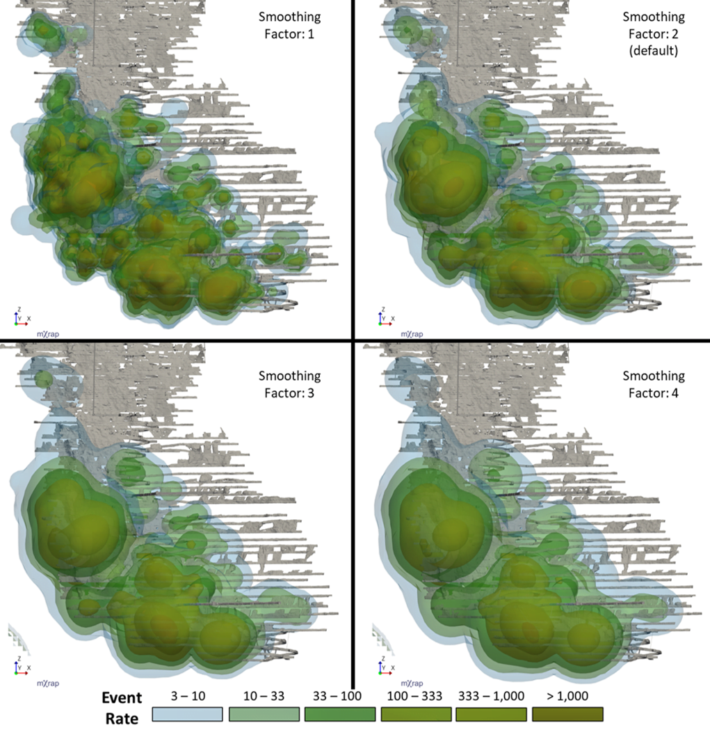
These parameters are capped at 100 m so Rmax can't go higher than that. There is a final smoothing factor applied to Rmax that is a control in the Advanced window. The default smoothing factor is to double the calculated Rmax. The figure below shows the effect of the smoothing factor on event rate at the Unicorn Gold mine. Increasing the smoothing factor generally lowers the peaks and raises the troughs of the event rate distribution throughout the mine.

Small Event Weighting

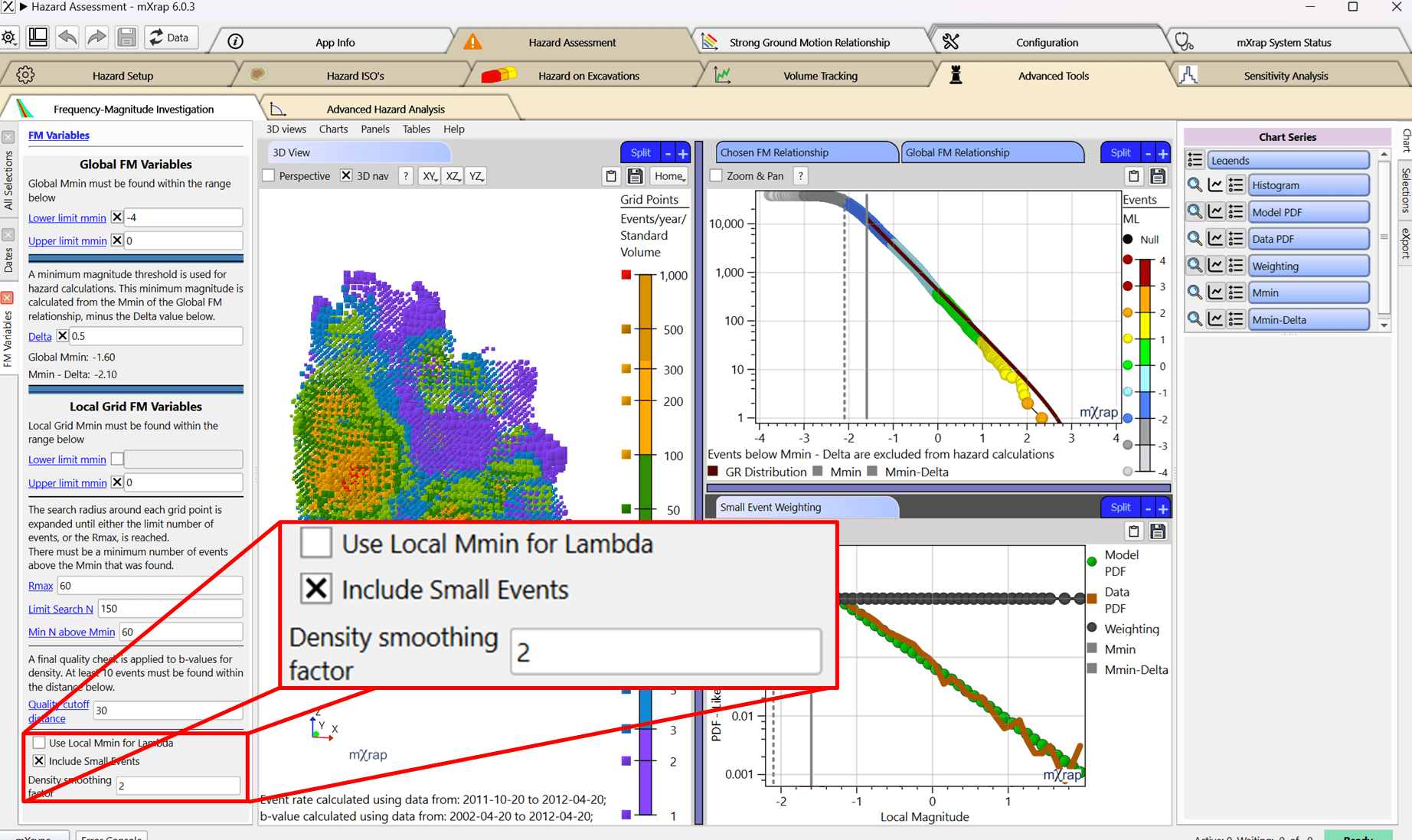
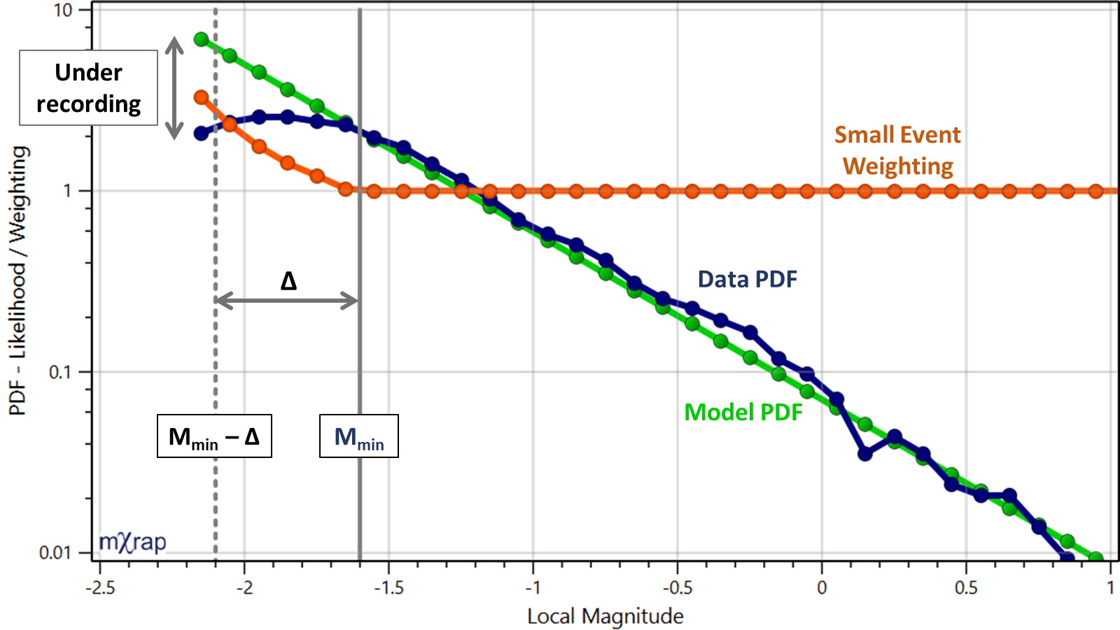
Event rate calculations generally use events above the global $Mmin$. The trouble is this excludes a significant portion of the database and limits the resolution of the seismic hazard assessment. To try and utilise additional data, events just below the global $Mmin$ are also considered. Events below $Mmin$ within a magnitude range, Δ, are splattered onto the grid as an alternate estimation of event rate. Since these events are under recorded, their contribution onto the grid is increased to compensate. The figure below shows how the small event weighting is calculated by estimating the amount of under recording compared to a complete dataset.

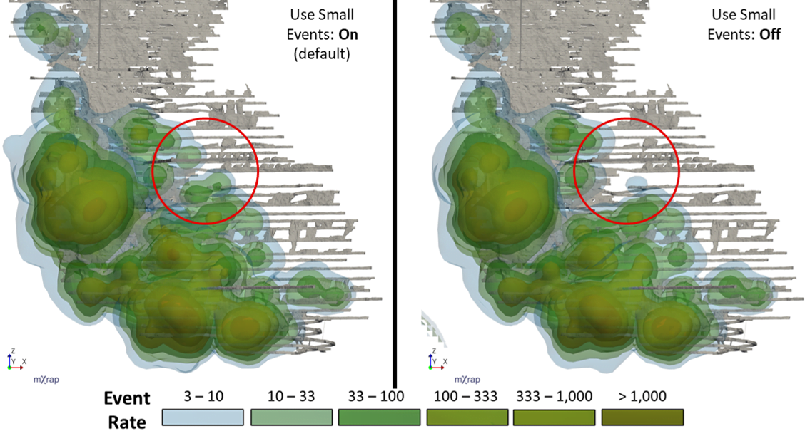
The two event rate calculations, from events above the global $Mmin$, and smaller events, are compared and the higher of the two rates is used. The use of smaller events is turned on by default, but you can turn this off in the Advanced window. You can see the difference in the event rate calculations at the Unicorn Gold mine with and without the small events. The differences are small but there is generally more information at the edges of the seismic clusters when small events are used.

Using Local Mmin

The event rate calculations generally don't consider the spatial variation in $Mmin$. However, we have made a recent addition to give you the option of using the local $Mmin$ calculated at each grid point. The same approach is taken, except an event is only splattered onto a grid point if its' magnitude is above the local $Mmin$. The small event adjustment still works but the global trend in under recording is used for the small event weightings.

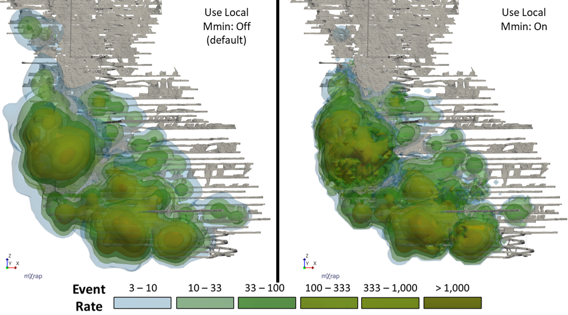
The local $Mmin$ option is available in the Advanced window and the results are compared for the Unicorn Gold mine below. The same general trends are there when using local $Mmin$ although it does increase the variability. The differences are more prevalent in areas with lots of data.

Concluding remarks

Feel free to investigate these event rate controls at your site and consider if they might be of use to you. In general, the differences will be small as the event rate is fairly insensitive to these variables but it will vary case-by-case. Remember that for hazard assessment, $b$-value is a far more sensitive parameter than event rate (previous post) so hopefully the decisions and assumptions made here won't have too much impact on your interpretations of hazard.